Notebook 5b: Ray-tracing projection on the GPU

Here we compare the CPU and GPU implementations of ray tracing projection.

Please see also notebook 5a.

This notebook requires that you have the GPU requirements installed and available on your system and that you have modified your Paicos user settings to load GPU functionality on startup. Please see the details here: https://paicos.readthedocs.io/en/latest/installation.html#gpu-cuda-requirements

import paicos as pa
import numpy as np
pa.use_units(True)

# Load snapshot
snap = pa.Snapshot(pa.data_dir, 247)

center = snap.Cat.Group['GroupPos'][0]
R200c = snap.Cat.Group['Group_R_Crit200'][0]
widths = np.array([10000, 10000, 10000]) * R200c.uq

# Pixels along horizontal direction
npix = 256

# Do some arbitrary orientation
orientation = pa.Orientation(normal_vector=[0, 0, 1], perp_vector1=[1, 0, 0])
orientation.rotate_around_normal_vector(degrees=20)
orientation.rotate_around_perp_vector1(degrees=35)
orientation.rotate_around_perp_vector2(degrees=-47)

# Initialize projectors
tree_projector = pa.TreeProjector(snap, center, widths, orientation, npix=npix,
                                  tol=0.25)

gpu_projector = pa.GpuRayProjector(snap, center, widths, orientation, npix=npix,
                                   threadsperblock=8, do_pre_selection=True,
                                   tol=0.25)

# Project density
tree_dens = tree_projector.project_variable('0_Density', additive=False)
gpu_dens = gpu_projector.project_variable('0_Density', additive=False)

Attempting to get derived variable: 0_Volume... [DONE]

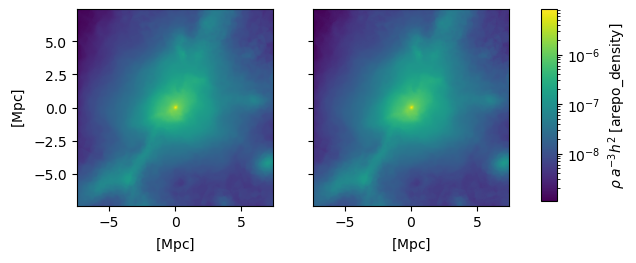
Plot comparison between CPU and GPU

%matplotlib inline
import matplotlib.pyplot as plt
from matplotlib.colors import LogNorm
plt.figure(1)
plt.clf()
fig, axes = plt.subplots(num=1, ncols=2, sharex=True, sharey=True)

extent = tree_projector.centered_extent.to_physical.astro.to('Mpc')
axes[0].imshow(tree_dens.value, extent=extent.value, norm=LogNorm(tree_dens.value.min(), tree_dens.value.max()))
im = axes[1].imshow(gpu_dens.value, extent=extent.value, norm=LogNorm(tree_dens.value.min(), tree_dens.value.max()))

# Add a colorbar
fig.subplots_adjust(right=0.8)
cbar_ax = fig.add_axes([0.85, 0.3, 0.025, 0.4])
cbar = fig.colorbar(im, cax=cbar_ax)

# Set the labels. The units for the labels are here set using the .label method
# of the PaicosQuantity. This internally uses astropy functionality and is
# mainly a convenience function.
cbar.set_label(tree_dens.label('\\rho'))
axes[0].set_ylabel(extent.label())
axes[0].set_xlabel(extent.label())
axes[1].set_xlabel(extent.label())

plt.show()